SDDP.jl - A Flexible SDDP Library
What we can do with it:
- Multistage stochastic linear program in discrete time
- RHS uncertainty (scenarios)
- Markov uncertainty
- Risk neutral or risk averse
What are we talking about
A stage has six things

- An incoming state $x_{t-1}$
- An outgoing state $x_t$
- Uncertainty that is realised at the beginning of the state $\omega_t$
- An action that is taken $u_t$
- Some dynamics $x_t = f_t(x_{t-1}, u_t, \omega_t)$
- A reward that is earned $c_t(x_{t-1}, x_t, u_t)$
$SP_t$ is a user defined JuMP model.
Where this might differ
- If I record 6 different states (initial, + five more), there are five stages, not six;
- Wait-and-See in a stage. You take an action today after realising the uncertainty(hazard-decision);
- Each stage is set-up as a linear programme.
We call the linear programme that defines a stage a subproblem.
# To get started we need to clone SDDP.jl
Pkg.clone("https://github.com/odow/SDDP.jl")

# load some packages
using SDDP, JuMP, Clp
The stock example
Links to StochDynamicPrograming.jl and SDDP.jl versions.
- Sense: Minimising
- Stages: 5 stages ($t = 1,2,3,4,5$)
- States: 1 State $x_t \in [0, 1]$ (initial state $x_0 = 0.5$)
- Controls: 1 control $u_t \in [0, 0.5]$
- Noises: 10 stagewise independent noises: $\omega_t \in [0, 0.0333..., 0.0666..., ..., 0.3]$
- Dynamics: linear dynamics $x_t == x_{t-1} + u_t - \omega_t $
- Stage Objective: linear objective $(\sin(3t) - 1) \cdot u_t$
Syntax for creating a new SDDPModel
We define 1. and 2. in the constructor using keyword arguments.
m = SDDPModel(
 sense = :Min,      # :Max or :Min?
 stages = 5,        # Number of stages
 solver = ClpSolver(),
 objective_bound = -2# Valid lower bound
 ) do sp, t
   # ) do subproblem_jump_model, stage_index
   # the first is a new JuMP Model for the subproblem, the second is an index from 1,2,...,5

 # ... subproblem definition goes here ...

end
Defining the subproblem
We still need to define the last five things:
3. States
4. Controls
5. Noises
6. Dynamics
7. Objective
We're going to use both sp and t from above.
3. Defining a state
A stage has an incoming, and an outgoing state variable. Behind the scenes we'll take care of matching them up between stages.
To define a new state variable use the @state macro.
@state(sp, lb <= outgoing <= ub, incoming == initial value)
First argument is the subproblem variable from the constructor, second argument is the outgoing variable (any feasible JuMP variable definition), third argument is the incoming variable (symbol == initial value).
From above, we have one state $x_t\in[0,1],\quad x_0 = 0.5$
@state(sp, 0 <= x <= 1, x0 == 0.5)
The x0 is the incoming variable in each stage. It will only be forced to 0.5 in the first stage. The syntax is just for convinence.
We could also create three state variables $x^i_t \in [0, \infty),\quad x^i_0 = i, \quad i=\{1,2,3\}\quad t=\{1,2,\dots,T\}$
@state(sp, x[i=1:3] >= 0, x0==i)
4. Defining a control
Controls are just JuMP variables. Nothing special.
From above $u_t \in [0, 0.5]$
@variable(sp, 0 <= control <= 0.5)
5. Defining a Noise
A noise has three things:
- A constraint
- A set of RHS values
- A probability distribution
Julia code is
@noise(sp, name = RHS Values, constraint)

setnoiseprobability!(sp, probability distribution)
From above we have
5 - Noises
- 10 stagewise independent noises: $\omega_t \in [0, 0.0333..., 0.0666..., ..., 0.3]$
6 - Dynamics
- linear dynamics $x_t == x_{t-1} + u_t - \omega_t $
@noise(sp, omega = linspace(0, 0.3, 10), x == x0 + u - omega)

# set uniform probability (but its the default so you don't have to
setnoiseprobability!(sp, fill(0.1, 10))
7. Defining the Stage Objective
We only care about defining the stage objective. The future costs get handled automatically.
stageobjective!(sp, AffExpr of Objective)
We can use the index t to change coefficients between subproblems so our objective is
stageobjective!(sp, (sin(3 * t) - 1) * u)
using SDDP, JuMP, Clp

m = SDDPModel(
                  sense = :Min,
                 stages = 5,
                 solver = ClpSolver(),
        objective_bound = -2
                                        ) do sp, t

    # the state
    @state(sp, 0 <= x <= 1, x0 == 0.5)

    # the control
    @variable(sp, 0 <= u <= 0.5)

    # the noise (and dynamics)
    @noise(sp, ω = linspace(0, 0.3, 10), x == x0 + u - ω)

    # the objective
    stageobjective!(sp, (sin(3 * t) - 1) * u)

end
Compare the Julia code to the mathematical subproblem
$ \begin{array}{r l} \min\limits_{u_t} & (sin(3t) - 1)u_t + \theta_{t+1}\\ s.t. & x_t = x_{t-1} + u_t - \omega_t \\ & x_t \in [0, 1] \\ & u_t \in [0, 0.5] \\ & x_0 = 0.5 \end{array} $
m = SDDPModel(
                  sense = :Min,
                 stages = 5,
                 solver = ClpSolver(),
        objective_bound = -2
                                        ) do sp, t
 @state(sp,    0 <= x <= 1, x0 == 0.5)
 @variable(sp, 0 <= u <= 0.5)
 @noise(sp, ω = linspace(0, 0.3, 10),
        x == x0 + u - ω)
    stageobjective!(sp, (sin(3t) - 1)*u )
end
Solve options
For a full list run julia>? SDDP.solve
status = solve(m,
    max_iterations = 10,
    time_limit     = 600,
    simulation     = MonteCarloSimulation(
                        frequency = 5,
                        min       = 10,
                        step      = 10,
                        max       = 100,
                        terminate = false
                    )
)
srand(1111)
status = solve(m,
    max_iterations = 20,
    time_limit     = 600,
    simulation     = MonteCarloSimulation(
                        frequency = 5,   # Number of forwards to construct the statistical bound
                        min       = 10,  # Min number of forwards to evaluate confidence interval for the bound
                        step      = 10,
                        max       = 100,
                        confidence = 0.95,
                        termination = false
                    ),
     print_level=0
)

# MonteCarloSimulation(frequency,steps,confidence,termination)
# MonteCarloSimulation(frequency,collect(min:step:max),confidence,termination)


# Check bound is correct
println("Final bound is $(SDDP.getbound(m)) (Expected -1.471).")
-------------------------------------------------------------------------------
                      SDDP Solver. © Oscar Dowson, 2017.
-------------------------------------------------------------------------------
    Solver:
        Serial solver
    Model:
        Stages:         5
        States:         1
        Subproblems:    5
        Value Function: Default
-------------------------------------------------------------------------------
              Objective              |  Cut  Passes    Simulations   Total
      Expected        Bound   % Gap  |   #     Time     #    Time    Time
-------------------------------------------------------------------------------
       -1.591         -1.471         |     1    0.0      0    0.0    0.0
       -1.365         -1.471         |     2    0.0      0    0.0    0.0
       -1.518         -1.471         |     3    0.0      0    0.0    0.0
       -1.624         -1.471         |     4    0.0      0    0.0    0.0
  -1.569    -1.479    -1.471   -6.7  |     5    0.0     20    0.0    0.1
       -1.537         -1.471         |     6    0.0     20    0.0    0.1
       -1.387         -1.471         |     7    0.1     20    0.0    0.1
       -1.403         -1.471         |     8    0.1     20    0.0    0.1
       -1.567         -1.471         |     9    0.1     20    0.0    0.1
  -1.491    -1.424    -1.471   -1.4  |    10    0.1    120    0.1    0.2
       -1.347         -1.471         |    11    0.1    120    0.1    0.2
       -1.456         -1.471         |    12    0.1    120    0.1    0.2
       -1.525         -1.471         |    13    0.1    120    0.1    0.2
       -1.801         -1.471         |    14    0.1    120    0.1    0.2
  -1.524    -1.453    -1.471   -3.6  |    15    0.1    220    0.2    0.3
       -1.746         -1.471         |    16    0.1    220    0.2    0.3
       -1.276         -1.471         |    17    0.1    220    0.2    0.3
       -1.285         -1.471         |    18    0.1    220    0.2    0.3
       -1.236         -1.471         |    19    0.1    220    0.2    0.3
  -1.505    -1.435    -1.471   -2.3  |    20    0.2    320    0.2    0.4
-------------------------------------------------------------------------------
    Statistics:
        Iterations:         20
        Termination Status: max_iterations
-------------------------------------------------------------------------------
Final bound is -1.4710749176074305 (Expected -1.471).simulation = simulate(m, 1000, [:x, :u])
println("Mean of simulation objectives is $(mean(r[:objective] for r in simulation))")
@visualise(simulation, i, t, begin
    simulation[i][:x][t], (title="State")
    simulation[i][:u][t], (title="Control")
    simulation[i][:scenario][t], (title="Scenario")
    simulation[i][:stageobjective][t], (title="Objective", cumulative=true)
end)
Example: Simplified Hydrothermal Dispatch
- Assume two thermoelectrics plants and one hydroelectric plant with reservoir and unit productivity coefficient.
- The first thermoelectric with cost 100 and the second with 1000 (R\$/ MWh) and capacities equal to 50 MW each.
- The hydroelectric plant has a reservoir with a capacity equivalent to 150 MWh that starts with a power of 150 MW.
- We want to minimize the cost of generating the next 3 hours.
- Demand is constant and equal to 150 MWh in all hours.
Notation
- $ g_{i, t}$ - thermoelectric generation
- $u_t$ - turbine
- $ v_t $ - reservoir volume
- $ a_t $ - affluence
- $ s_t $ - spillway
Subproblem
$FCF(v_{t-1}) =$
\begin{array}{r l} \min\limits_{g,s,u,s \geq 0} & 100 g_{1,t} + 1000 g_{2,t}\\ s.t. & g_{1,t} + g_{2,t} + u_t = 150 \\ & v_t + u_t + s_t = v_{t-1} + a_t \\ & 0 \leq v_t \leq 200 \\ & 0 \leq u_t \leq 150 \\ & 0 \leq g_{1,t} \leq 50 \\ & 0 \leq g_{2,t} \leq 50 \\ \end{array}m = SDDPModel(
sense = :Min,
stages = 3,
solver = ClpSolver(),
objective_bound = 0
) do sp, t
# State
@state(sp, 0 <= v <= 200, v0 == 50)
# Variables
@variable(sp, 0 <= g[1:2] <= 100)
@variable(sp, 0 <= u <= 150)
@variable(sp, s >= 0 )
# Noise
@noise(sp, a = linspace(50, 0, 10), v + u + s == v0 + a)
# Constraints
@constraint(sp, g[1] + g[2] + u == 150)
# Objective function
stageobjective!(sp, 100*g[1] + 1000*g[2] )
end
srand(1111)
status = solve(m,
    max_iterations = 20,
    time_limit     = 600,
    simulation     = MonteCarloSimulation(
                        frequency = 5,
                        min       = 10,
                        step      = 10,
                        max       = 100,
                        termination = false
                    ),
     print_level=0
)

println("Final bound is $(SDDP.getbound(m)) (Expected 57470).")
# Simulation
simulation = simulate(m, 1000,[:g, :u])
println("Mean of simulation objectives is $(mean(r[:objective] for r in simulation))")
Average Value at Risk
risk_measure = NestedAVaR(lambda = 0.5, beta = 0.5)
A risk measure that is a convex combination of Expectation and Average Value @ Risk (also called Conditional Value @ Risk).
lambda * E[x] + (1 - lambda) * AV@R(1-beta)[x]
Keyword Arguments
lambda- Convex weight on the expectation ((1-lambda)weight is put on the AV@R component. Inreasing values oflambdaare less risk averse (more weight on expecattion)beta- The quantile at which to calculate the Average Value @ Risk. Increasing values ofbetaare less risk averse. Ifbeta=0, then the AV@R component is the worst case risk measure.
m_risk = SDDPModel(
                  sense = :Min,
                 stages = 5,
                 solver = ClpSolver(),
           # risk_measure = Expectation(),
           risk_measure = NestedAVaR(lambda=0.5, beta=0.5),
        objective_bound = 0
                                        ) do sp, t

    # the state
    @state(sp, 0 <= x <= 1, x0 == 0.5)

    # the control
    @variable(sp, 0 <= u <= 0.5)

    # the noise (and dynamics)
    @noise(sp, omega = linspace(0, 0.3, 10), x == x0 + u - omega)

    # the objective
    stageobjective!(sp, (sin(3 * t) - 1) * u)

end
println(typeof(m_risk))
srand(1111)
status = solve(m_risk,
    max_iterations = 20,
    time_limit     = 600,
    simulation     = MonteCarloSimulation(
                        frequency = 5,
                        min       = 10,
                        step      = 10,
                        max       = 100,
                        termination = false
                    ),
    print_level=0
)

# Check bound is correct
println("Final bound is $(SDDP.getbound(m_risk)).")
De Matos (Level One) Cut Selection
m_risk = SDDPModel(
                  sense = :Min,
                 stages = 5,
                 solver = ClpSolver(),
           risk_measure = Expectation(),
        objective_bound = -2,
        cut_oracle      = DematosCutOracle()
                                        ) do sp, t
Asyncronous Solver
We parallelise by farming out a new instance of the SDDPModel to all slave processors.
Slaves perform iterations independently, and asyncronously share cuts between themselves.
solve(m,
    solve_type = Serial()
    # or
    solve_type = Asyncronous()
)
Markov Uncertainty
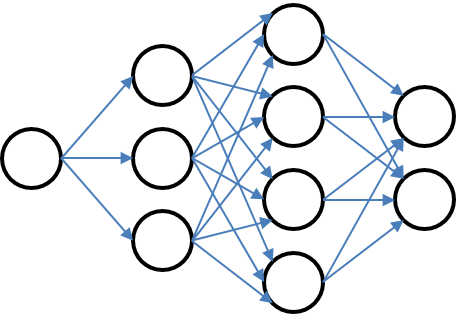
More like a feed-forward graph with discrete stages but arbitrary number of nodes and transitions

# Transition[last index, current_index] = probability
Transition = Array{Float64, 2}[
    [1.0],
    [0.5 0.5],
    [0.25 0.75; 0.75 0.25],
    [0.25 0.75; 0.75 0.25],
    [0.25 0.75; 0.75 0.25]
]
Transition = Array{Float64, 2}[
    [1.0]',
    [0.5 0.5],
    [0.25 0.75; 0.75 0.25],
    [0.25 0.75; 0.75 0.25],
    [0.25 0.75; 0.75 0.25]
]

m_markov = SDDPModel(
                  sense = :Min,
                 stages = 5,
                 solver = ClpSolver(),
        objective_bound = -10,
        # A vector of transition matrices. One for each stage
      markov_transition = Transition
                                        # markov_state will go from 1, 2, ..., S
                                        ) do sp, t, markov_state
    @state(sp, 0 <= x <= 1, x0 == 0.5)
    @variable(sp, 0 <= u <= 0.5)
    @noise(sp, omega = linspace(0, 0.3, 10), x == x0 + u - omega)

    # the objective
    stageobjective!(sp, (sin(3 * t) - 0.75 * markov_state) * u)

end
println(typeof(m_markov))
status = solve(m_markov,
    max_iterations = 10,
    print_level=0
)

# Check bound is correct
println("Final bound is $(SDDP.getbound(m_markov)).")